In this blog post, I want to give you a gentle introduction to text classification.
Text classification (also known as text categorisation or text tagging) is the process of mapping natural language text to pre-defined categorical variables.
There are many applications for text classification, such as spam detection and sentiment analysis. Understanding these concepts is crucial for engaging in a Deep Dive into Language Learning Models ‘LLM’, which can further illuminate the complexities of intent detection and other classifications.
In a previous blog post, I went over some important machine learning concepts like train-test splits, cross-validation, and accuracy measurements, and showed how to implement a Naïve Bayes classifier in a few lines of code using scikit-learn. In this blog post, I want to dive a bit deeper into the maths and show you how linear classification algorithms work.
Let’s take text classification based on topics as an example — like categorising news articles by their content: sports, politics, and technology. In this case, grammar does not matter and the core signal you get in order to make classification is the words being used. Hence, a sophisticated model that takes syntactic and semantic features into account is not necessary, and a linear model is appropriate for this task.


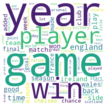
The three-word clouds above highlight the most common words based on frequency and relevance for the three types of news articles, named above.
So if you see a new piece of text where the words “game”, “season” and “played” come up more often than the words “online” and “network”, the news article is most likely about sports.
Below you see the vectors for a hypothetical news article for each group using a bag-of-words approach. In the previous article of this series, I wrote about how to extract features from text and represent human language text as computer-readable vectors. Now we will use those extracted features to predict whether a news article is about sports or not (we will treat this problem as a binary prediction task for now).
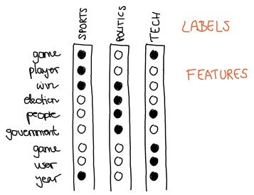
In supervised machine learning, you have input features and sets of labels.
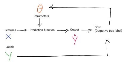
To make predictions based on your data, you use a function F with some parameters Θ to map your features to output labels. To get an optimum mapping from your features to labels, you minimise the cost function which works by comparing how closely your output Ŷ is to the true labels Y from your data. Learning takes place by updating the parameters and repeating the process until your cost is minimised.
What to expect
I will go over two important algorithms: logistic regression and Naive Bayes. Both algorithms, despite being relatively simple, often produce good results and are good algorithms to start with. They are often used as baselines for comparison to more sophisticated approaches. Another reason why these two algorithms are often presented together is to demonstrate the difference between discriminative (logistic regression) and generative classifiers (Naive Bayes). These are two very different frameworks for how to build a machine learning model.
Consider a visual metaphor: imagine we are trying to distinguish elephant images from lion images. A generative model would have the goal of understanding what elephants look like and what lions look like. You could, hypothetically, ask that model to ‘generate’ (i.e. draw) an elephant. Given a test image, the system then asks whether it is the elephant model or the lion model that better fits the image, and chooses that as its label.
A discriminative model, by contrast, is only trying to learn to distinguish the classes. Elephants have trunks and lions do not. If that one feature neatly separates the classes, the model is satisfied. But if you ask such a model what it knows about lions, all it can say is that they do not have trunks.
Logistic Regression
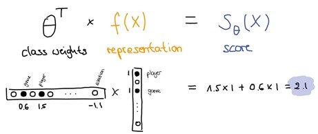
Let’s take a hypothetical sports vector representing a news article about sports and multiply this vector with a vector of class weights that we have learned during the training phase, where each word in the vocabulary has a weight. This weight indicates whether it is useful to have this particular word in the given class. In this example, “player” with a weight of 1.5 means that it is most likely a “sports” word, whereas “election” with a weight of -1.1 most likely is not. And the score is a dot product of these two vectors.
Discriminative classification tries to find a line (hyperplane) that separates the classes the best. To visualise it in 2-dimensional space: each dot is a feature representation of a news article. The weight vector is a vector that is orthogonal to this hyperplane that separates the sports from the non-sports articles. And the score is the projection of the feature vector (the dot in space) on the weight vector minus the bias term (intercept). So you see that this dot product does exactly what we need as it draws the hyperplane between the sports and the non-sports instances.

Once we have these scores, the next step is to assign probabilities to these scores
At the moment these scores can be anything between minus infinity to plus infinity. We do not need this in order to do predictions on our test set — the scores are sufficient in order to tell whether an article is about sports (positive score) or not (negative score). However, this mapping to probabilities is important during training in order to quantify our loss.
This is where the sigmoid function comes in handy — it squashes minus infinity to plus infinity into a space between zero and one, which is exactly what we need to get a probability. And then what we have is the probability of a particular sentence being labelled as “sports”, conditioned on the sentence’s content x to be the sigmoid function applied to the score of x:
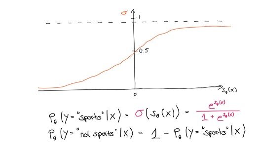
And it follows that the probability of non-sports is 1 minus the probability of sports. Now we choose the label with the highest probability and assign that label to the article. We use the hat notation ^ to mean “our estimate of the correct class”.
ŷ = argmax PΘ(y|x) y ϵ {sports, not sports}
If you have a multiclass problem (Sports, Politics, Technology) the softmax function is used instead of the sigmoid.
Now let us consider the loss function
During training, we will have some training loss. This training loss is defined in terms of a training dataset (in our case, our news articles) where we have pairs of x and y, where x are the articles and y are the topic labels. And the training loss is the aggregate loss over all the instances (articles) in our training data. For each instance, we have an instance-specific loss which basically checks, given the current model parameters, how good the prediction is compared to the true label.
The loss function used for logistic regression is called negative log-likelihood.
Where Dataset: D = (x1, y1) … (xn, yn)
Loss: L(D,Θ) = 1/n l(xi, yi, Θ) (l = per instance loss)
Conditional log likelihood: l(x,y,Θ) = -log pΘ(y|x)
Intuitively it means that my loss is low if for each of the training instances the gold label y has a high probability. So the higher the probability of the actual training labels for the training instances, the lower the loss. The reason for the minus sign is because optimisation usually minimises a function, so maximising the likelihood is the same as minimising the negative likelihood.
By updating the parameters of the model during training in order to minimise the loss, the weight vector that we talked about is learned. The optimisation algorithm used for that is called gradient descent. It is out of the scope of this blog to cover gradient descent separately, but the idea is to take baby steps in the opposite direction of the gradient of the function at the current point (because this is the direction of the steepest descent) until you arrive at a minimum, where the loss is the smallest.
I will conclude my gentle introduction to logistic regression for text classification. I can highly recommend this video series about logistic regression, this video about gradient descent, and this chapter of the book “Speech and Language Processing” by Daniel Jurafsky and James H. Martin.
Naive Bayes
Let us now look at the Naive Bayes classifier. It is a simple classifier based on probabilities of events. Like above, we want to maximise the probability of the predicted class c given the input d (d for document).
ĉ = argmax PΘ(c|d) c ϵ C
The intuition of Bayesian classification is to use Bayes’ rule to transform the equation above into their probabilities that have some useful properties.

We then substitute the first equation into the second one to get:

We can conveniently simplify the above equation by dropping the denominator P(d). This is possible because we will be computing P(d|c)P(c) / P(d) for each possible class, but P(d) does not change for each class; we are always asking the most likely class for the same article d, which must have the same probability P(d). Thus, we can choose the class that maximises the simpler formula

Generative Model
Now you can see how Naive Bayes is a generative model: because we can read the above as stating a kind of implicit assumption about how a document is generated: first a class is sampled from P(c), and then the words are generated by sampling from P(d|c). At this point, we could imagine generating artificial documents, or at least their word counts, following this process.
We choose the probable class ĉ given some article d by choosing the class which has the highest product of two probabilities: the prior probability P(c) and the likelihood of the article P(d|c). The article is represented as a set of features: x = (f1, f2, f3….fn).
Here, we have already made one simplifying assumption by using the bag-of-words model which assumed that the position of the word does not matter. The second simplifying assumption that Naive Bayes makes is the conditional independence assumption of the probabilities P(fi|c) given a class c. Namely, NB assumes that the individual words are independent of each other (hence NAIVE Bayes), and the likelihood can therefore be calculated as

The final equation for the class chosen by a naive Bayes classifier is thus:
Let’s go over a numerical example.
Consider the following sentences:
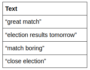
To make the example easier to follow, let’s assume we applied some pre-processing to the sentences and removed stopwords. The resulting sentences are:
Total words for class “sports”: 3
Total words for class “not sports”: 4
At this point, we want to assign a class to the following sentence “that was a very close and memorable match”. After stop word removal: “close memorable match”.
We can see that the priors for both classes are the same:
P(Sports) = 0.5
P(Not Sports) = 0.5
likelihood P(“close memorable match”|Sports) = P(“close”|Sports) * P(“memorable”|Sports) * P(“match”|Sports)
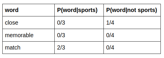
Now we run into a problem
Because the words “close” and “memorable” are not in the vocabulary of the sports class we end up with 0 when multiplying the individual probabilities. The simplest solution is the add-one (Laplace) smoothing: we are adding 1 to the numerator and the number of words in the total vocabulary to the denominator. This results in the following values:

likelihood P(“ close memorable match”|Sports) = 1/10 * 1/10 * 3/10 = 0.003
likelihood P(“ close memorable match”|not Sports) = 2/11 * 1/11 * 1/11 = 0.0015
Posterior = likelihood * prior, so the probability of the sentence “that was a very close and memorable match” belonging to the class “sports” is 0.0015, whereas the probability belonging to the class “not sports” is 0.00075. So the sentence gets labelled as “sports”.
I strongly encourage you to read this chapter of the book “Speech and Language Processing” by Daniel Jurafsky and James H. Martin, as it does not only cover Naive Bayes but also metrics for evaluating text classification.
I hope you found this blog post useful and got a better understanding of how logistic regression and Naive Bayes work for text classification. You obviously do not have to implement these algorithms from scratch, as all machine learning libraries for Python have already done that for you. However, it is important to understand how they work in order to understand their benefits and potential weaknesses so that you can design a model that works the best for your particular type of data or problem.

AUTHOR: Lisa A Chalaguine – SheCanCode Blog Squad


