

Data Visualization is an important step in machine learning. Data Visualization is used to visualize the distribution of data, the relationship between two variables, etc.
So, let’s take a deep dive into univariate and bivariate analysis using seaborn.
Univariate Analysis
- Histogram
- Distplot
- Box plot
- Countplot
Bivariate Analysis on Categorical Variables
- Barplot
Bivariate Analysis on Continuous Variables
- Scatterplot
- lmplot
- lineplot
- regplot
I have taken the Iris data set and have performed univariate and bivariate analysis of it.
Univariate Analysis
-
Histogram
A histogram is a visualisation tool that represents the distribution of one or more variables.
sns.histplot(df[“sepal length”],color=‘darkorange’)
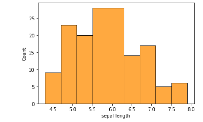
From the above histogram plot, we can infer that the sepal length ranges from 4 to 8. And also we can infer that more iris species have sepal length between 5.5 to 6.5.
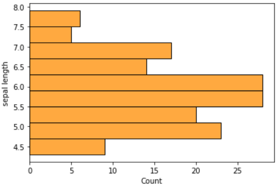
To get vertical histogram plots, we can switch the axis.
sns.histplot(y=“sepal length”,data=df,color=‘darkorange’)
Histogram for categorical variables
To include ‘cat2egorical variables’, the hue parameter is used. The color encoding is done based on the categorical variable.
sns.histplot(x=‘sepal length’,data=df,hue=df[‘iris’])

From the plot, we can infer the sepal length of various ‘iris’ species.
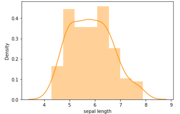
2. distplot
Distplot is a histogram with a line on it. Displot is used for single variable distribution.
sns.distplot(df[“sepal length”],color=‘darkorange’)
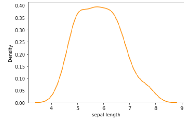
To visualize distplot alone, we can give hist=False
sns.distplot(df[“sepal length”],hist=False,color=‘darkorange’)
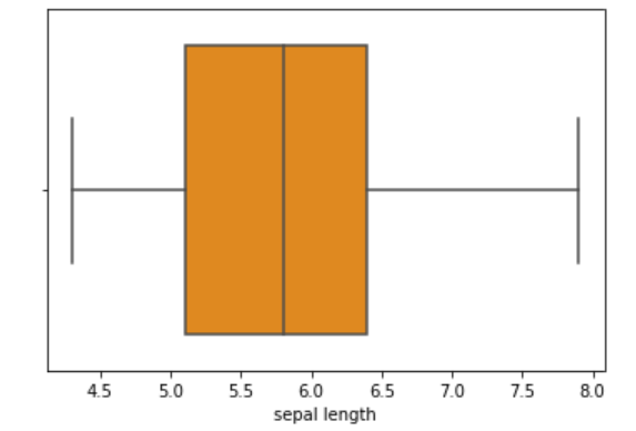
3. Boxplot
Box plot is used to visualize the descriptive statistics of a variable. It is used to detect outliers. It represents the five-point summary.
Five Point Summary
min,max,median,lower quartile(Q1),upper quartile(Q3)
sns.boxplot(df[“sepal length”],color=’darkorange’)
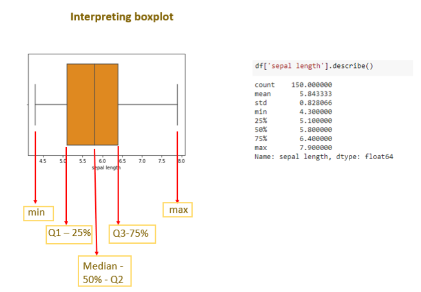
Interpreting boxplot
Boxplot is the pictorial representation of descriptive statistics.
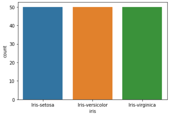
4. countplot
Count plot is used for the distribution of categorical variables. It shows the count of each categorical bin.
sns.countplot(df[‘iris’])
Bivariate Analysis on Categorical Variables
-
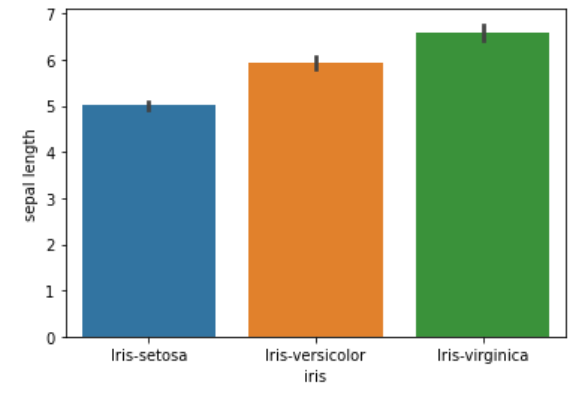
Barplot
Barplot is used to aggregate the categorical data based on some aggregate methods. By default it is mean.
sns.barplot(x=‘iris’,y=‘sepal length’,data=df)
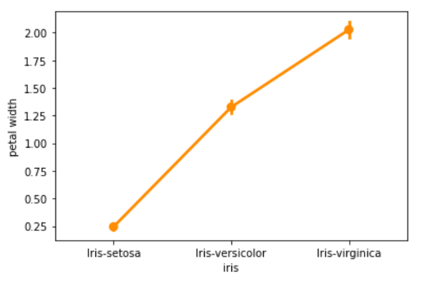
2. pointplot
Pointplot helps to visualize the distribution of values at each level of the categorical variable.
sns.pointplot(x=‘iris’,y=‘petal width’,data=df,color=‘darkorange’)
Bivariate Analysis on Continuous Variables
-
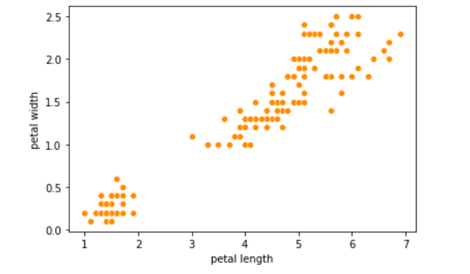
scatterplot
The scatterplot shows the correlation between two numerical variables.
sns.scatterplot(df[“petal length”],df[‘petal width’],color=‘darkorange’)
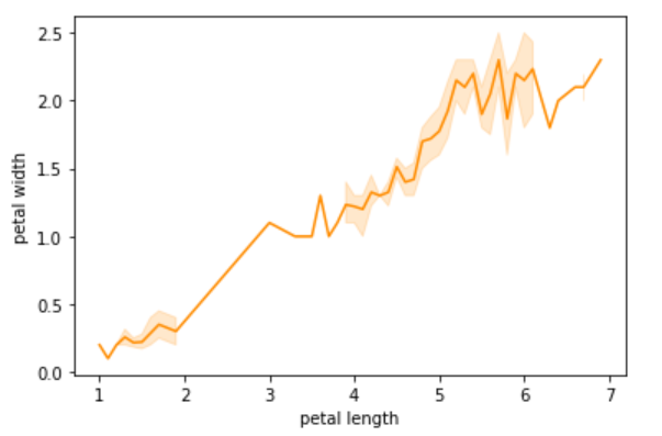
2. lineplot
The relationship between two numerical variables is shown in a line.
sns.lineplot(df[‘petal length’],df[‘petal width’],color=‘darkorange’)
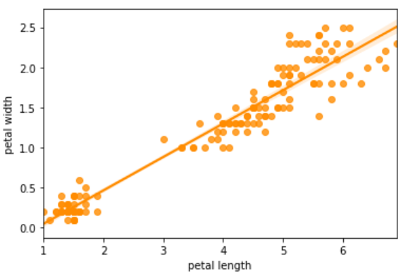
3. regplot
Regplot is a scatterplot with a regression line to it.
sns.regplot(df[‘petal length’],df[‘petal width’],color=‘darkorange’)
Conclusion
In this article, I have covered the different types of univariate and bivariate analysis using the iris data set. Thanks for reading!